Introduction :
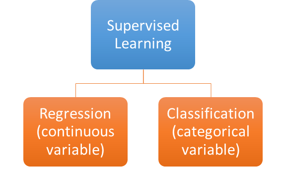
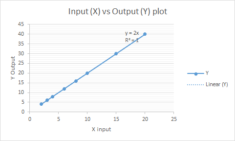
Linear regression is basically a supervised learning algorithm to predict continuous (any numerical value) target values based on a given set of input variables. If we plot the approximate line/plane on a 2D- 3D graph it would have a constant slope.
Types of Linear Regression :
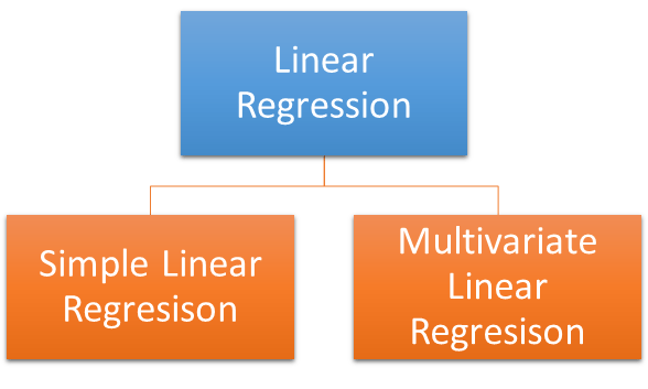
Simple linear regression:
Its the basic slope intercept form of a line in a 2D plane.
y = m*x + b
“y” is the predicted variable, “m” is the slope and “b” is the intercept and “x” is the input variable.
Multivariate Regression:
Multivariate regression comes into play when more than one input variable/feature/attribute is used for prediction, unlike the simple linear regression.
f(x,y,z) = w1*x +w2*y + w3*z + b
Here, x, y, z are the input features, b is the bias and w1, w2, w3 are the weights/coefficients which the machine decides to predict the best output value.
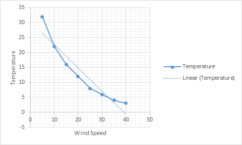
Example:
Temperature = w1 * Wind-speed + Bias
Bias is intercept in this case. i.e where the line intersects the Y- axis.
So, this all seems very basic , but even now we have not come to the concept of “learning”. How does the machine actually learn from this? The basic concept for any machine to learn is to minimize a Cost function/ Loss function.
What is a Cost/Loss function ?
Cost function measures the performance of a machine learning model. It can be different based on the given problem or data set . It also quantifies the difference between the predicted and actual value. In a sense we need to be very close to the predicted value or in the best of cases reduce the cost function down to zero.
So, coming back to the cost function specific to linear regression we concentrate on Mean Squared Error (MSE):
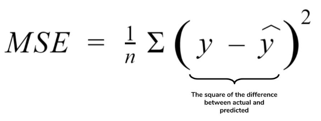
Here, Y hat is the predicted value and Y is the actual value, n is the number of observations in the data set.
So how do we reduce the cost function? How does the machine calculate optimal values of bias and coefficients to reduce the cost function ? We need another technique to teach the machine how to reduce the cost function.
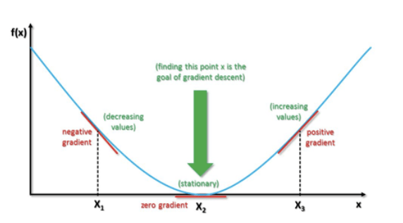
Gradient Descent :
Gradient descent is a technique which helps reduce the cost function. It helps the machine to find the optimal coefficients and bias.
https://srdas.github.io/DLBook/GradientDescentTechniques.html
The curve at any position can be called as a gradient. Now, the goal is to reach the bottom most position of the function where the gradient or slope equals to zero. A broad overview is to select random values(0 or any small value) of the coefficients and calculate the gradient for the function by using those values. We calculate this by using the derivative of the function. Check the cost at each step for minimum. Keep iterating this till the time the machine is not able to reduce the cost function any further.
Steps for Gradient Descent :
Step 1 : Set initial value of the coefficients. Zero or any random small value.
Step 2 : Calculate the cost function using the initial values of the coefficients.
Step 3: Calculate the derivative of the cost function. i.e the slope at that point of the gradient. Check if the slope is positive or negative.
delta = deriv(cost func)
Step 4 : Modify the coefficients as per the slope direction( positive or negative). Here, a learning rate parameter(alpha) is added to control how much a coefficient value needs to be changed.
coef = coef – (alpha * delta)
Step 5: Iterate till the cost reaches zero or close to zero.